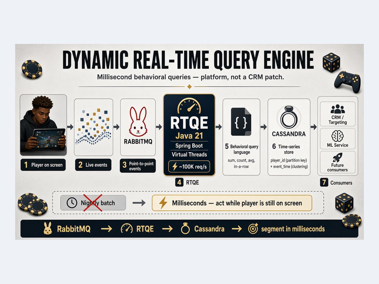
Every gaming company will tell you the same thing – the difference between a player who stays and a player who leaves is often decided in a matter of seconds. In that window, the right message, the right offer, or the right nudge can change the entire trajectory of a relationship. Miss it, and the moment is gone.
For us, that window wasn’t seconds. It was milliseconds.
In 2025, I led the architecture for a system we came to call the Dynamic Real-Time Query Real – Time Query Engine — a platform that lets our CRM and marketing teams understand a player’s behavior the instant an event happens and act on it while the player is still on screen. No nightly batch jobs. No “we’ll reach them tomorrow.” Just live behavior, computed and acted upon in real time.
It started, as many good systems do, with a problem nobody could solve. Our CRM team had spent six months trying to make existing tools do something they were never designed for. When they hit a wall, the problem landed on the desk of the Architecture Board and that’s where my part of the story begins.
This article is about how we got from “this is impossible with what we have” to a production system answering behavioral queries in milliseconds. I’ll walk through the problem, the architecture we designed, the trade-offs we wrestled with, and the lessons I took away from leading the effort — both the technical ones and the human ones this — the problem ones and the human ones.
If you build real-time systems, work in data infrastructure, or care about CRM and marketing technology, I hope you’ll find something useful here.
The Decision: Build a Platform, Not a Patch
When my solution architects, the VP of Engineering, the CTO, and I sat down to brainstorm, the easy path would have been to bolt yet another point solution onto the CRM stack. We chose not to.
The key realization in that room was this — the problem the CRM team brought us wasn’t really a CRM problem — it was a data problem. The CRM tools couldn’t act in milliseconds because nothing in our stack could answer questions about a player’s live behavior fast enough. Solve that, and we wouldn’t just unblock CRM – we’d unlock a whole class of real-time use cases.
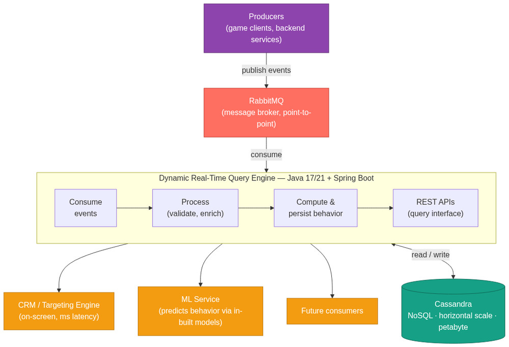
So we decided to build the Dynamic Real-Time Query Engine as a foundational building block – a piece of platform infrastructure, not a feature. The same engine that resolved the CRM problem could serve several consumers at once:
The CRM / targeting engine- segment players in real time and trigger on-screen treatments within milliseconds of an event.
The ML Service- act as a real-time data provider, feeding live behavioral features into in-built ML models that predict what a player is likely to do next.
Future consumers - any team that needs to ask fast questions about live player behavior, without building their own pipeline.
This reframing changed everything. Instead of designing a narrow tool for one team, we were designing a shared real-time data and query layer that the whole business could build on. It raised the stakes and the scope – but it was the right call.
The Tech Stack (and Why We Chose It)
Architecture is ultimately a series of trade-offs, and the technology choices are where those trade-offs become concrete. Here’s what we picked and the reasoning behind each decision.
Java 21 - the core language
We built the engine on Java, running on Java 21. For a system that has to process a high volume of events concurrently while keeping latency low, Java was a natural fit:
– It’s a mature, battle-tested language for large-scale backend systems, with a rich ecosystem and tooling.
– Its multithreading and concurrency support is first-class - exactly what we needed to fan out work and squeeze every millisecond out of the hardware.
Spring Boot - the application framework
On top of Java, we used Spring Boot to build the service layer. It gave us:
A fast path to production-grade REST APIs, so consumers (CRM, the ML Service, the targeting engine) could integrate over a clean, well-understood interface.
Built-in support for the operational concerns that matter in production - configuration, dependency injection, metrics, health checks without reinventing the wheel.
Cassandra - the storage engine
For storage we chose Apache Cassandra, a distributed NoSQL database. Given our requirements, this was one of the most important decisions we made:
Horizontal scalability. Cassandra scales out by simply adding nodes, with no single point of failure – essential for a system expected to grow with player volume.
Petabyte scale capacity. It’s designed to store and serve enormous datasets, so we wouldn’t hit a ceiling as event volume exploded.
Write and read-friendly at scale. Its architecture suits a high-ingest, high-query workload like ours, where events stream in constantly and consumers query live behavior just as constantly.
A traditional relational database would have struggled with this combination of write throughput, data volume, and the need for predictable performance under load. NoSQL – specifically Cassandra was the right tool for the job.
RabbitMQ - the message broker
To move events from producers into the engine, we used RabbitMQ as our message broker, following a point-to-point communication model:
A producer emits an event (a player action) onto a queue.
The query engine consumes that event, processes it, and persists the result into Cassandra.
This decoupling was important. The producer doesn’t need to know anything about how the engine works, how busy it is, or whether it’s momentarily slow – it just publishes. RabbitMQ buffers the events and hands them to the engine to consume at its own pace, which keeps the pipeline resilient under bursty load and gives us a clean seam between event production and event processing.
The Data Model
If the architecture is the skeleton, the data model is the heart of the engine. In Cassandra, your data model is your performance -you model around the queries you need to answer, not around some abstract notion of “clean” relational design. This is where we spent a disproportionate amount of our thinking, and it paid off.
One table per event type, modeled as a time series
We made two deliberate decisions:
1. One Cassandra table per event type. Each kind of player event gets its own table, rather than cramming every event into a single generic table. This keeps each table’s schema tight, its partitions predictable, and its queries fast.
2. Model every event table as a time series. Player behavior is inherently a sequence of events over time, so we leaned into Cassandra’s strength: time-series data keyed by entity.
This time-series design plays a crucial role in how the engine performs. It lets us answer the question that matters most - what has this player been doing recently?” - by reading a single, contiguous slice of one partition.
The key design
For each event table, the primary key is structured as:
Partition key: `player_id` - all of a player’s events of a given type live together on the same node, so reading one player’s recent activity is a single-partition lookup (the fastest thing Cassandra can do).
Clustering key: event timestamp- events are physically ordered by time within the partition, so “the last N events” or “events in the last X milliseconds/minutes/hours/days” is a cheap, sorted range scan.
Remaining columns: the event’s attributes- whatever payload that event type carries.
A representative table looks like this:
CREATE TABLE game_result_events (
  player_id text,
  event_time timestamp,
  game_id text,
  rake double,
  winning_amt double,
  is_winner text,
  PRIMARY KEY ((player_id), event_time)
) WITH CLUSTERING ORDER BY (event_time DESC);
A deliberate constraint: a small, fixed set of data types
We made one more rule that surprised people: across the entire engine, we restricted attribute data types to a small, fixed set`double`, `text`, and `timestamp`.No nested collections, no exotic types - just the primitives we actually needed (whole numbers, monetary/decimal values, strings, and time).
This was a conscious trade-off in favor of speed, simplicity, and predictability:
A simpler, uniform schema is far easier to validate, serialize, and query consistently across hundreds of event tables.
Predictable storage and parsing- a handful of primitive types means no surprises in how data is stored, indexed, or deserialized on the hot path.
Fewer foot-guns- restricting types kept producers honest and prevented a long tail of edge cases that would have slowed the engine and complicated the code.
Constraints like this are easy to undervalue, but in a system optimizing for millisecond latency, every bit of uniformity you can buy is latency you don’t have to fight for later.
The Query Language: A JSON DSL for Behavior
Here’s where the “query engine” really earns its name. Rather than forcing the CRM and marketing teams to write SQL – or worse, to file engineering tickets every time they wanted a new segment we built our own JSON-based query language.
The goal was simple: let non-engineers (and other services) express rich behavioral questions as data, not code. A query is just JSON, so it can be created in a UI, stored, versioned, sent over an API, and evaluated by the engine in real time.
What the language supports
The DSL is small but expressive. It covers the operations that behavioral targeting actually needs:
Aggregate functions:`sum`, `count`, `avg` (average), `max`, `min`, `uniqueCount`, and an in-a-row (consecutive streak) aggregate.
Comparison conditions:`gt` (greater than), `gte` (greater-or-equal), `lt`, `lte`, `eq` (equals), `noteq` (not equals), and `eqic` (equals, ignore case).
Logical / arithmetic operators: `and`, `or`, `nor`, and a `compare` operator for relating one computed value to another.
A query is built from two parts:
1. queryModels - one or more named sub-queries (`q1`, `q2`, …). Each model computes a single aggregate over a single event table, optionally filtered by a time window and `WHERE`- style conditions.
2. expression- an optional layer that combines the results of those models with conditions and logical operators, turning several aggregates into one true/false segment decision.
Anatomy of a query model
Each model has a consistent shape:
"q1": {
"queryData": {
"rake": {
"value": "0",
"cond": "gt",
"function": "sum",
"searchTime": {
"cond": "days",
"from": "600",
"toDate": ""
},
"queryWhereEvent": [
{ "whereColumn": "game_type", "whereCond": "eqic", "whereValue": "Stake" },
{ "whereColumn": "server_type", "whereCond": "eqic", "whereValue": "Stake" },
{ "whereColumn": "bet", "whereCond": "gte", "whereValue": "10" }
]
}
},
"tableName": "player_games"
}
In plain English, `q1` asks: “Over the last 600 days, for this player’s `player_games` events where `game_type` and `server_type` are ‘Stake’ (case-insensitive) and `bet >= 10`, is the sum of rake` greater than 0”
Notice how much is packed into one declarative block: the table, the aggregate, the time window (which maps directly onto our time-series clustering key), and the row filters. The engine translates this into an efficient, single-partition, time-bounded scan over Cassandra.
Composing models into a segment
The real power shows up when you combine multiple models with an `expression`. Here’s a segment built from five sub-queries, all over a 7-day window:
Each model produces a number; the `expression` block then thresholds and combines them. Read together, this query targets a specific kind of high-value player in the last 7 days:
{
"queryModels": {
"q1": { "queryData": { "wagering": { "function": "sum", "cond": "gt", "value": "0", "searchTime": { "cond": "days", "from": "7" }, "queryWhereEvent": [] } }, "tableName": "rummy_game_dtls" },
"q2": { "queryData": { "win_loss_status": { "function": "count", "cond": "eq", "value": "Won", "searchTime": { "cond": "days", "from": "7" }, "queryWhereEvent": [] } }, "tableName": "rummy_game_dtls" },
"q3": { "queryData": { "bet": { "function": "count", "cond": "eq", "value": "500", "searchTime": { "cond": "days", "from": "7" }, "queryWhereEvent": [] } }, "tableName": "rummy_game_dtls" },
"q4": { "queryData": { "deposit_amt": { "function": "sum", "cond": "gt", "value": "0", "searchTime": { "cond": "days", "from": "7" }, "queryWhereEvent": [] } }, "tableName": "add_cash_status" },
"q5": { "queryData": { "redeemed_amt": { "function": "sum", "cond": "gt", "value": "0", "searchTime": { "cond": "days", "from": "7" }, "queryWhereEvent": [] } }, "tableName": "player_redeem_status" }
},
"expression": {
"q1": { "cond": "gt", "value": "10000", "arthOperator": "and" },
"q2": { "cond": "gte", "value": "1" },
"q3": { "cond": "gte", "value": "1", "arthOperator": "and" },
"q4": { "cond": "gte", "value": "5000" },
"q5": { "cond": "gte", "value": "2500", "arthOperator": "and" }
}
}
q1: total `wagering` > 10,000, and
q2: won at least 1 game (`count` of `Won` ≥ 1), and
q3: placed a bet of 500 at least once (`count` ≥ 1), and
q4: deposited at least 5,000, and
q5: redeemed at least 2,500.
One JSON document, evaluated across three different event tables, becomes a precise, real-time audience definition the CRM team can act on instantly.
Going further: comparing computed values
The language can also relate values to each other, not just to constants, using the `compare` operator. For example:
{
"queryModels": {
"q1": { "queryData": { "wagering": { "function": "avg", "cond": "gt", "value": "0", "searchTime": { "cond": "days", "from": "30" }, "queryWhereEvent": [] } }, "tableName": "rummy_game_dtls" },
"q2": { "queryData": { "redeemed_amt": { "function": "sum", "cond": "gt", "value": "0", "searchTime": { "cond": "days", "from": "30" }, "queryWhereEvent": [] } }, "tableName": "player_redeem_status" }
},
"expression": {
"q1": { "cond": "gt", "value": ["wallet_balance", "500"], "arthOperator": "compare" },
"q2": { "cond": "gte", "value": ["q1"], "arthOperator": "compare" }
}
Here the `value` is an array, and `compare` lets the engine evaluate one quantity against another – comparing `q1` against a `wallet_balance` (and `500`), and then `q2` against the result of `q1`. This is what makes the language dynamic: expressions can reference other columns and even other query results, not just hard-coded numbers.
Why build our own language?
It’s a fair question - why not just expose SQL? A few reasons drove the decision:
Safety and control. A constrained DSL can’t issue an unbounded or accidentally catastrophic query. Every model maps to a bounded, single-partition, time-windowed read by construction.
It speaks the domain. “Sum of rake over 600 days where game_type is Stake” is closer to how the CRM team thinks than raw SQL joins.
It’s portable data. Because a query is just JSON, it can be authored in a UI, stored, shared, A/B tested, and replayed by humans or by the ML Service.
It maps cleanly onto our data model. The `searchTime` window lines up with the time-series clustering key, and `tableName` with our one-table-per-event-type design, so every query has an efficient execution path.
Optimization: Parallelism, Thread Starvation, and Virtual Threads
A query that touches one table is easy. But our real queries like the five – model segment earlier fan out across multiple tables, columns, and date ranges in a single request. Doing that one model at a time would have been far too slow for millisecond targeting. This is where the optimization work began.
Step 1: Understand the query before you run it
Before executing anything, the engine scans the incoming query first to segregate exactly what work needs to be done - the distinct tables, columns, and date ranges each model requires. Knowing the full shape of the work up front let us plan the reads intelligently instead of discovering them as we went.
Step 2: Parallelize across tables
With the work mapped out, we ran a separate thread for each table, using Java’s `CompletableFuture` to execute the model reads concurrently and then join all the results back together. Instead of paying the latency of each Cassandra read in series, we paid roughly the cost of the slowest one. Leveraging parallelism this way was the single biggest lever for keeping multi-model queries fast.
Step 3: Hitting the wall - thread starvation at 100K req/s
This worked beautifully… until it didn’t. As traffic climbed to around 100K requests per second, we started seeing query execution slow down - not because Cassandra was struggling, but because of thread starvation.
The problem was structural. With classic platform threads, every concurrent table read consumed an OS thread from a bounded pool. At 100K req/s, each spawning multiple `CompletableFuture` tasks, the pool simply couldn’t keep up - requests queued waiting for a thread to free up, and latency spiked. We were starving for threads, not for CPU or database capacity.
Step 4: Java 21 virtual threads
This is where the move to Java 21 virtual threads paid off. Virtual threads are lightweight, JVM-managed threads that aren’t pinned 1:1 to OS threads, so you can have a very large number of them in flight at once. The blocking Cassandra reads that previously tied up scarce platform threads now ran on cheap virtual threads instead.
The effect was dramatic: queries that had been backing up under thread starvation executed seamlessly, because thread availability was no longer the bottleneck. We got the simple, readable blocking-style concurrency model and the scalability to handle the load.
Step 5: Taming the memory spike with ZGC
Virtual threads solved the thread starvation, but they introduced a new symptom: with so many threads in flight at once, each holding its own stack and short-lived objects, we saw memory usage spike under heavy load. More concurrency meant more allocation pressure, and that put more work on the garbage collector.
The fix was to switch to ZGC (the Z Garbage Collector). ZGC is a low-latency, concurrent collector designed to handle very large heaps while keeping pause times in the sub-millisecond range – it does most of its work concurrently with the application instead of stopping the world. Even when virtual threads pushed memory up, ZGC reclaimed it very fast and without the long GC pauses that would have eaten into our millisecond latency budget. Virtual threads gave us the concurrency; ZGC kept that concurrency from turning into latency.
Step 6: Scale out, not just up
Finally, the engine runs as a containerized service that autoscales. When request volume surges, more instances spin up to share the load; when it subsides, they scale back down. Combined with virtual threads handling concurrency within each instance, this gave us headroom both vertically (per instance) and horizontally (across instances).
Tuning Cassandra for Real-Time Reads
Parallelism and virtual threads got the application tier out of the way - but the engine is only as fast as the database underneath it. Getting Cassandra to serve recent player behavior with predictable, low latency took deliberate tuning.
Caching the hot path: row cache and key cache
Our access pattern is heavily skewed toward recent data most queries ask about what a player did in the last few minutes, hours, or days. That makes caching enormously effective:
Key cache keeps partition-key locations in memory, so Cassandra can skip straight to the right data on disk instead of hunting for it.
Row cache keeps the actual hot rows in memory, so repeated reads of a player’s latest events are served without touching disk at all.
Together these dramatically speed up recent reads (and writes) exactly the rows our real-time queries hit most often. For a workload like ours, where the “last N events for this player” is asked over and over, the cache hit rate is high and the latency win is real.
Compaction: time-window strategy + TTLs
The second big lever was compaction strategy. Because every event table is a time series and we attach a TTL to events (they age out automatically once they’re no longer relevant), we chose a time-based / time-window compaction strategy rather than the default size-tiered approach.
This pairing is a natural fit:
Events written in the same time window are compacted together into the same SSTables.
When those events expire via TTL, whole SSTables can be dropped at once, instead of expired data lingering and being repeatedly rewritten.
That means far less wasted compaction work - and, crucially, less garbage-collection pressure on the JVM, which keeps latency steady and avoids GC pauses creeping into our millisecond budget.
Results
When the dust settled, the Dynamic Real-Time Query Engine delivered on the promise that started it all:
Millisecond query latency. Behavioral questions that used to be impossible in real time are now answered in milliseconds, fast enough to act on a player while they’re still on screen.
Scale we can grow into. After the move to Java 21 virtual threads, the engine sustains around 100K requests per second, with containerized autoscaling absorbing traffic spikes and Cassandra giving us horizontal, petabyte-scale headroom for event volume.
One engine, many consumers. What began as a CRM problem became shared infrastructure – powering the CRM and targeting engine, and serving as a real-time data provider for the ML Service that predicts player behavior.
Self-serve for the business. The CRM team now defines brand-new behavioral segments in JSON and puts them live in minutes, with no engineer in the loop.
What I learned leading the architecture
The technology was the fun part, but leading the effort taught me just as much.
Reframe the problem before you solve it. The CRM team handed us a CRM problem. The moment we recognized it was really a data problem, the solution stopped being a patch and became a platform. The most valuable work happened in that reframing – in the room with the CTO and VP – before any code was written.
Constraints are a feature. Restricting the type system, building a bounded JSON DSL instead of exposing raw SQL, modeling one table per event type – each of these removed options on purpose. Those constraints are exactly what kept the engine fast, safe, and predictable under load.
Make the data model the first decision, not the last. In a real-time system, the partition key, clustering key, compaction strategy, and TTL aren’t tuning details you bolt on at the end – they’re the foundation the millisecond latency rests on.
Your bottleneck is rarely where you think. At our peak load we assumed the database was the limit. It wasn’t – it was our threading model. Measuring carefully, rather than guessing, is what pointed us at virtual threads instead of throwing more Cassandra nodes at the problem.
Raise the level of abstraction for the people you serve. The biggest win wasn’t any single optimization – it was handing the business a language to ask its own questions. Great infrastructure makes other teams faster without making them wait on you.
Conclusion
We set out to solve a problem nobody else could crack: understanding a player’s behavior the instant it happened and acting on it within milliseconds. What we built was bigger than the original ask – a Dynamic Real-Time Query Engine that turns live player events into answers fast enough to change outcomes in the moment.
The pieces all reinforce one another. A time-series data model in Cassandra, keyed by player and ordered by time. A small, safe JSON query language that lets the business express rich behavioral questions as data. Parallel, virtual-thread-powered execution that scales to roughly 100K requests per second. Caching and time-window compaction that keep the hot path in memory and let old data evaporate cleanly. Every decision points in the same direction – toward predictable, low-latency answers at scale.
But the real lesson is one that outlasts any particular stack: the best architecture doesn’t just solve the problem in front of you – it reframes that problem into a capability the whole business can build on. A CRM team’s six-month headache became a foundational platform that now powers targeting, machine learning, and whatever comes next.
If you’re tackling something similar – real-time systems, behavioral data, or just the messy art of leading an architecture from a whiteboard to production – I’d love to compare notes.
Wrapping Up
To recap the journey in one place:
The problem: a gaming CRM team needed to compute player behavior from a live event and act on the player, on screen, within milliseconds – something existing CRM tools couldn’t do.
The decision: instead of patching CRM, we built the Dynamic Real-Time Query Engine as a shared platform building block that also feeds the ML Service and the targeting engine.
The stack: Java 21 and Spring Boot for the engine, RabbitMQ for point-to-point event delivery, and Cassandra as a horizontally scalable, petabyte-scale NoSQL store.
The data model: one table per event type, modeled as a time series with player_id as the partition key and event_time as the clustering key, using a small fixed set of data types.
The query language: a JSON DSL with aggregates (sum, count, avg, max, min, uniqueCount, in-a-row), conditions (gt, gte, lt, lte, eq, noteq, eqic), and operators (and, or, nor, compare) – composed from queryModels and an expression.
The performance: query-aware parallelism with CompletableFuture, Java 21 virtual threads to beat thread starvation at ~100K req/s, autoscaling containers, plus Cassandra row/key caching and time-window compaction with TTLs.
The outcome: millisecond behavioral queries at scale, and a self-serve platform the business builds new segments on in minutes.
If there’s one thing to take away: the best architecture doesn’t just solve today’s problem – it turns that problem into a capability the whole organization can build on.